Para facilitar la exposición nos concentraremos en el caso
univariado (![]() ). El caso multivariado es completamente análogo.
). El caso multivariado es completamente análogo.
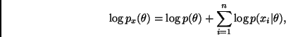
Sea
![]() y denotemos por
y denotemos por
![]() a la moda de
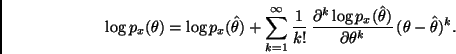
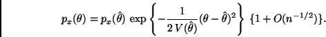
a la moda de ![]() . Desarrollando
. Desarrollando
![]() en serie de Taylor alrededor de
en serie de Taylor alrededor de ![]() tenemos
tenemos
Por otra parte, notemos que
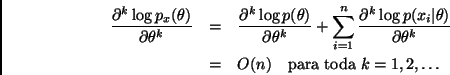
Ahora, sea
Por otro lado, como consecuencia del Corolario 2.1 tenemos que
Comentario. Recordemos que
![]() . Tenemos entonces
que la desviación estándar asintótica,
. Tenemos entonces
que la desviación estándar asintótica,
![]() , es de orden
, es de orden
![]() . Así, las aproximaciones se requieren solamente en
regiones tales que
. Así, las aproximaciones se requieren solamente en
regiones tales que
![]() es de orden
es de orden ![]() ,
puesto que fuera de estas regiones
,
puesto que fuera de estas regiones
![]() es
(asintóticamente) muy pequeña.
es
(asintóticamente) muy pequeña.
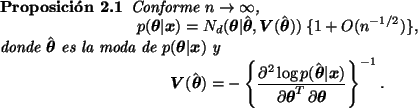
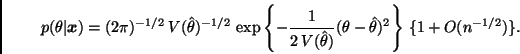
En el caso multiparametral, un argumento análogo permite demostrar la
siguiente versión de la aproximación normal asintótica a la
distribución final de
![]() .
.
Si esta aproximación es adecuada, entonces prácticamente cualquier
resumen inferencial de interés (e.g. distribuciones marginales o
momentos de funciones lineales de
![]() ) puede aproximarse
fácilmente. En particular,
) puede aproximarse
fácilmente. En particular,